Applying Game Theory to Traffic - El Farol Bar Problem
Why is Traffic So Unpredictable? An Application of the El Farol Bar Problem
2021-06-30
Note: This blog post includes an interactive Jupyter notebook with simulations written in Python. You can click the launch binder badge below to open the notebook in an executable environment and mess around with the simulations right away!
If there’s one thing we can all agree on, it’s that traffic sucks. Growing up in Colorado, I’ve experienced the torment of weekend ski traffic up in the mountains a lot more than I cared to.
Worth it though…
It’s especially irritating when you try to account for the traffic by leaving a bit earlier or later than usual and still end up stuck, potentially for hours. Through this painful ordeal one realizes that previous experience with traffic is insufficient to predict how bad it will be on any individual day. Of course short-term and long-term trends can arise for particular locations or times (the roads heading to the ski slopes during the winter are always busy, during the summer much less so), but day to day the number of drivers on any given road appears highly unpredictable. This is due to the large number of independent agents who have to make the decision to drive on the same road at the same time. Traffic is then seen as an emergent property that arises from the collective presence of a sufficient number of drivers on the road at once.
Before driving, a driver considers the information they know about the traffic along their route and determines whether or not the drive is worth it to them, without knowledge of what the other drivers are deciding (hence the term independent agents). This interplay between many interacting agents is comparable to stock market speculation, where a large number of independent traders have access to the same information (the stock’s performance over time) and make decisions about whether to buy or sell a business’s stock based on that information. The price at which a willing buyer and seller agree to trade at any time determines the stock price. The traditional economic approach treats the traders as perfectly rational, logical beings who will mitigate losses and take advantage of favorable circumstances. But is the decision making process in either of these scenarios actually perfectly rational?
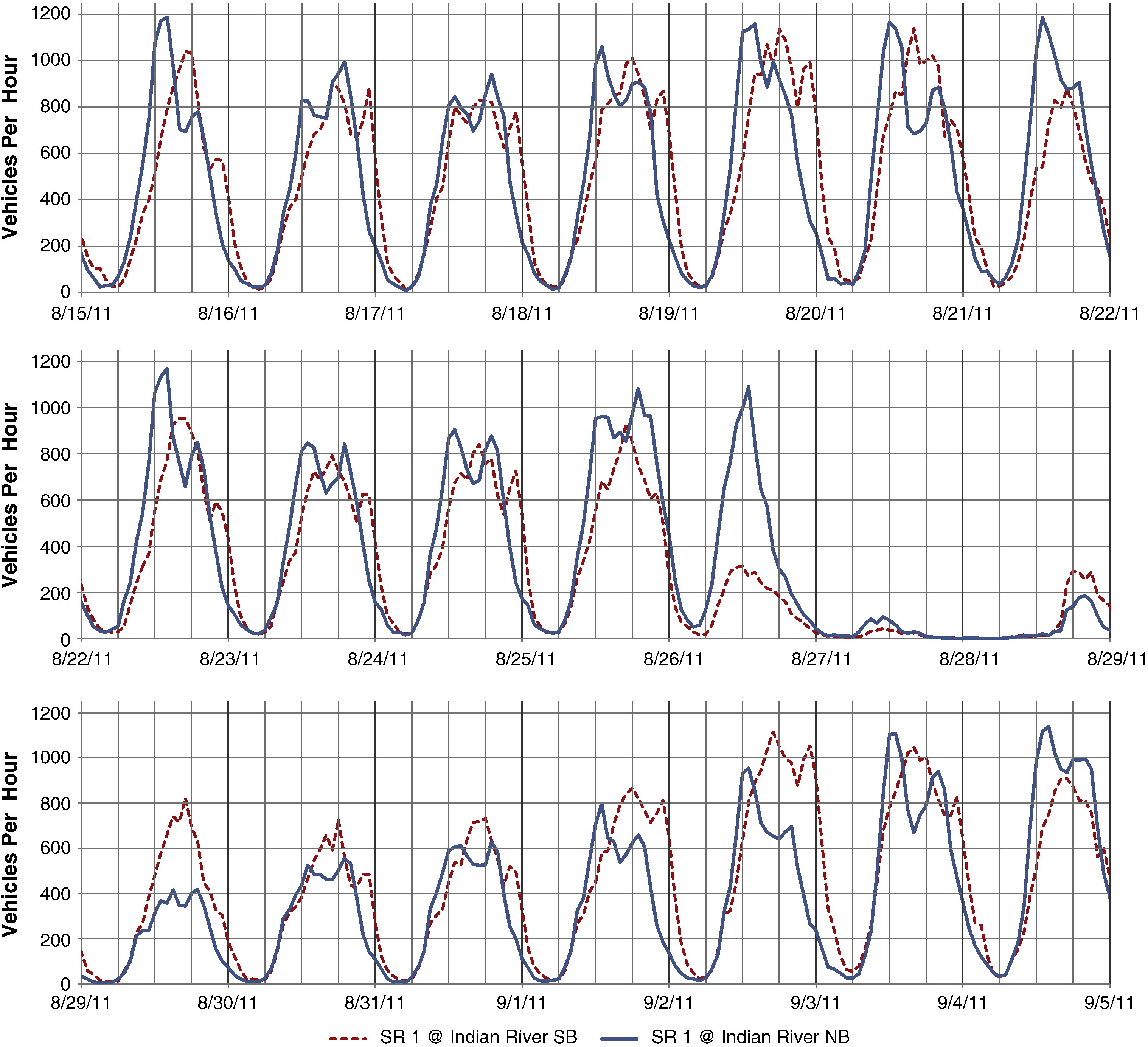 Hourly highway traffic data on Route 1 in Delaware taken before, during, and after Hurricane Irene in August 2011. The blue line represents northbound traffic, and the dashed red line is southbound traffic. Note the recurring patterns of low traffic during late night/early morning and high traffic around noon and the end of the work day, and how those patterns were almost entirely eliminated during the hurricane. Figure reproduced from [4] under a Creative Commons license. Copyright © 2012 International Association of Traffic and Safety Sciences. Published by Elsevier Ltd.
When faced with complicated or ill-defined situations, human deductive reasoning where one starts with a set of premises and uses logic to come to a conclusion that is necessarily true from those premises falls short. In the case of our traffic example, the fact that there are many other independent drivers playing the same game as you - and I’m using the word game in the technical sense, as we’ll see in a bit - means that it is by definition impossible to anticipate and account for what they are going to decide as part of your strategy. The information available to you is incomplete and you can’t depend on other people making perfectly rational decisions, hence perfect rationality with “objective, well-defined, shared assumptions” goes out the window [1]. Instead in such a situation modern psychology says that people will resort to inductive reasoning based on pattern recognition, hypothesis formation and testing, and adjusting hypotheses as needed, which humans are extremely good at [3]. You look at the previous days’ numbers, try to extrapolate trends, and if those trends fail you then you’re less likely to rely on them when forming your strategy next time. How would one go about modeling inductive reasoning in a situation with a large number of interacting agents, like drivers on a highway or traders in the stock market?
Modeling Inductive Reasoning with The El Farol Bar Problem
Economist and complexity theorist W. Brian Arthur was concerned about this same question of modeling inductive reasoning when he wrote his 1994 paper “Inductive Reasoning and Bounded Rationality” [1]. In the paper, he describes how inductive behavior among a collection of independent agents could be modeled by assuming that each agent can form several beliefs or mental models which are typically subjective (differing among the agents) and are subject to changes in the weights placed on those beliefs as the agents act upon the currently most believable or seemingly profitable model and keep track of the performance of each of their models. These models can come in many forms for different people, from if-then statements, simple mathematical equations, “just a feeling”, and more complicated statistical hypotheses. Regardless of the specific models used, the agents learn from the track record of their models and adjust them; personal models are constantly battling to prove themselves temporarily useful amongst a background environment of other models from other agents and the space of mental models in use by all of the agents coevolves [1]. Still, to apply this framework to a particular problem one must specify a well-defined system for generating the models.
To provide a concrete example illustrating inductive reasoning Arthur constructed a scenario which is now known as the El Farol Bar Problem, inspired by the bar El Farol in Santa Fe which offered Irish music on Thursday nights that apparently drew a big crowd. Sounds like a good time! Here’s Arthur’s original statement of the problem [1]:
“N people decide independently each week whether to go to a bar that offers entertainment on a certain night. For concreteness, let us set N at 100. Space is limited, and the evening is enjoyable if things are not too crowded-specifically, if fewer than 60 percent of the possible 100 are present. There is no sure way to tell the numbers coming in advance; therefore a person or agent goes (deems it worth going) if he expects fewer than 60 to show up or stays home if he expects more than 60 to go. Choices are unaffected by previous visits; there is no collusion or prior communication among the agents; and the only information available is the numbers who came in past weeks.”
At the individual level, the problem boils down to a decision between going to the bar and staying at home. From the collection of all such decisions comes the attendance number, and as the agents adjust strategies based on previous attendance one might expect the attendance to turn out random. However, in numerous different circumstances and realizations of the problem the mean attendance converges to the bar capacity [2, 5, 7]. Do you see why I’m bringing this up in relation to our traffic problem? Let’s return to that problem and simplify it, at least for now. Assume that we have N potential drivers who are contemplating driving on Highway 1 at some particular day and time each week, and the only information they have about the traffic is the previous d weeks’ numbers at the same time of day and day of the week. Also assume that traffic occurs if more than m out of the N drivers is on the road, and a driver will stay home if they expect traffic but will otherwise drive on Highway 1. Finally we assume that each week’s traffic numbers are known by everybody after the fact, even the people who decided not to drive that week. I will address some of the shortcomings of these assumptions at the end of this post, but for now we will use them to make the problem tractable.
Under these assumptions, our traffic scenario becomes the El Farol Bar Problem! Note that we posed the traffic problem as a week-to-week decision to align it with Arthur’s original framing of the El Farol Bar Problem, but we could have also said that the drivers make their decision on a day-to-day basis without any difficulty. We now just need to specify a system for generating and updating the models for each of the agents and then we can simulate what the numbers on the road each week look like over time.
Describing Traffic With Game Theory
This leads us to game theory, where we will consider the problem of driving on Highway 1 for a given week to be a one shot strategic game with a set of N players. “One shot” means that the game is played only once for the week, at the particular time of day and day of the week that we’re concerned with. Each player has a finite set of decisions (drive or not drive) and strategies for determining their decision, and a payoff function dependent on both an individual’s decision and the state of the traffic [2]. The week-to-week traffic scenario represented by the El Farol Bar Problem is then the repeated version of this one shot game for however long you want to look at the dynamics.
Our drivers make their initial guesses about how the traffic will be and act based on those guesses, and as time passes they learn from their experiences and adjust their strategies. From our assumption about the traffic history being available to everyone afterwards, we will say that a driver is happy with their decision in two of the four possible outcomes of the week:
- If they chose to drive and ≤ $m$ people drove in total (no traffic).
- If they chose not to drive and ≥ $m$ people drove in total (traffic).
Denoting the decision to drive by $x=1$ and the decision to stay home by $x=0$, and letting $n$ be the actual number of drivers who drive on the week ($n$ ≤ $N$), this corresponds to the following payoff function [5]:

The drivers in our model will be given a set number $k$ of strategies (or “predictors” in Arthur’s original language [1]) picked randomly from a finite list of functions that map traffic histories to a prediction about the traffic that week. These strategies include:
- Predict the average of the previous weeks’ traffic
- Predict the same traffic as last week (or as 2 weeks ago, or 3 or 4)
- Predict the standard deviation of the previous traffic, or $N$ minus the standard deviation if the attendance increased from two weeks ago to last week
- Mirror the attendace around $N$/2 from last week for a prediction; in this case 35 percent of people showing up last week corresponds to a prediction of 65 percent of maximum traffic numbers this week.
A full list of the 13 strategies available in our model is provided in the attached interactive Jupyter Notebook here. You’ll need to wait for it to load and then select “El Farol Bar Problem.ipynb” if you want to run the simulations yourself. In game theory the four strategies listed above are considered pure strategies because they provide a deterministic choice between the decisions (drive or stay home in this case) for any values of the traffic history - the same input data would lead to the same decisions [7]. Such strategies are to be contrasted with mixed strategies which are probability distributions over the decisions [6], with the most extreme example being a totally random guess about the traffic extracted from a discrete uniform distribution. We will consider what happens when drivers apply exclusively pure strategies, when they all randomly guess, and when there is a combination of pure and mixed strategies present.
The drivers aim to maximize their utility function each week and will change the strategy that they employ if their utility is zero at the end of a week. If none of their strategies would have given a utility of 1 the driver randomly picks one of the $k$ strategies that they know, but otherwise they randomly choose from the set of strategies that would have maximized their utility.
Simulation Results
Pure Strategies and Nash Equilibria
Before we dive into the full simulation results, we should think about what we expect to occur. An optimal result would be for each player to maximize their utility. To do so requires exactly $m$ players to decide to drive and $N-m$ to stay home, so that nobody would elect to change their strategies if they knew what everybody else was going to decide. Such a set of strategies where nobody has a unilateral incentive to deviate from their own strategy is known as a Nash equilibrium in game theory, named after legendary economist and mathematician John Nash [6]. More specifically the optimal situation in the full El Farol Bar Problem is a weak Nash equilibrium, where the word “weak” means that some driver may have multiple strategies which would result in the same utility if they switched between them while everyone else kept the same strategy. If each driver would suffer a loss in utility by switching their strategy while everyone else stayed fixed, the equilibrium would instead be considered a strong Nash equilibrium.
The number of weak pure-strategy Nash equilibria in our one shot strategic game is by definition the number of different sets of pure strategies that the $N$ players could pick which are Nash equilibria. We consider two sets of strategies to be different if at least one player changes their decision about driving from one set to the next; the different Nash equilibria correspond to swappings of the player’s decisions so that the $m$ people who drive changes. Therefore the number of weak pure-strategy Nash equilibria is the number of ways $m$ drivers can be selected out of the group of $N$ players,
\begin{aligned} {N\choose m} = \frac{N!}{m!(N-m)!}. \end{aligned}
Outcomes with these Nash equilibria are Pareto efficient in that no other outcome increases at least one player’s payoff without decreasing anyone else’s, but they are clearly unfair because only the same $m$ people get to drive each week [5]. The results of a simulation for one such pure strategy Nash equilibrium in the El Farol Bar Problem are shown below, with $N = 10000$ and $m = 0.6N$. This specific implementation has $m$ people always guess that 20% of the $N$ total players will show up (so those $m$ people always choose to go), and the remaining $N−m$ people always guess that 70% of the $N$ players will go (so they never show up).
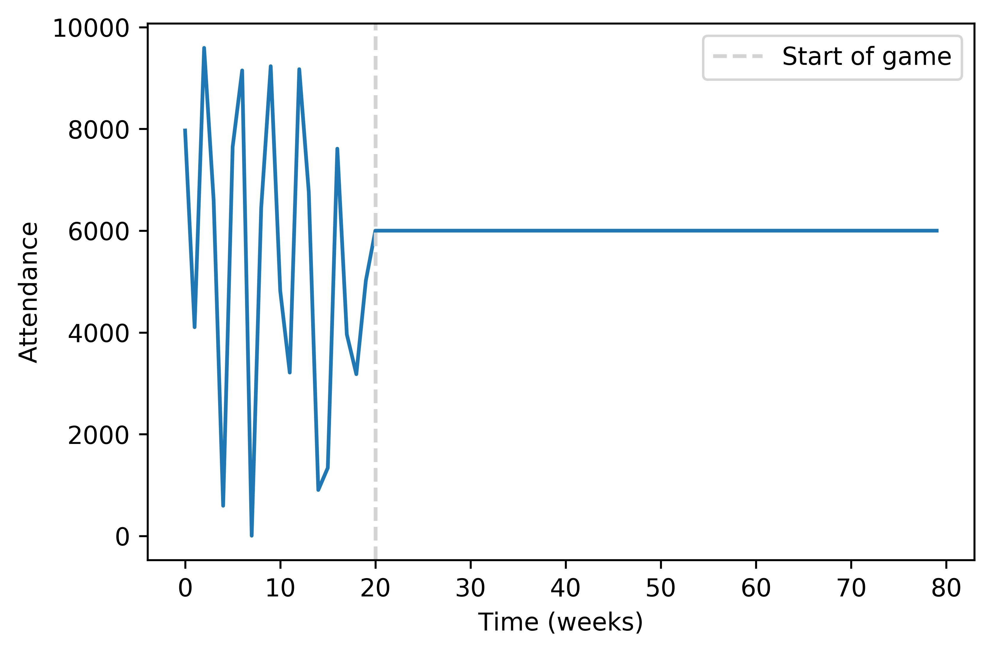
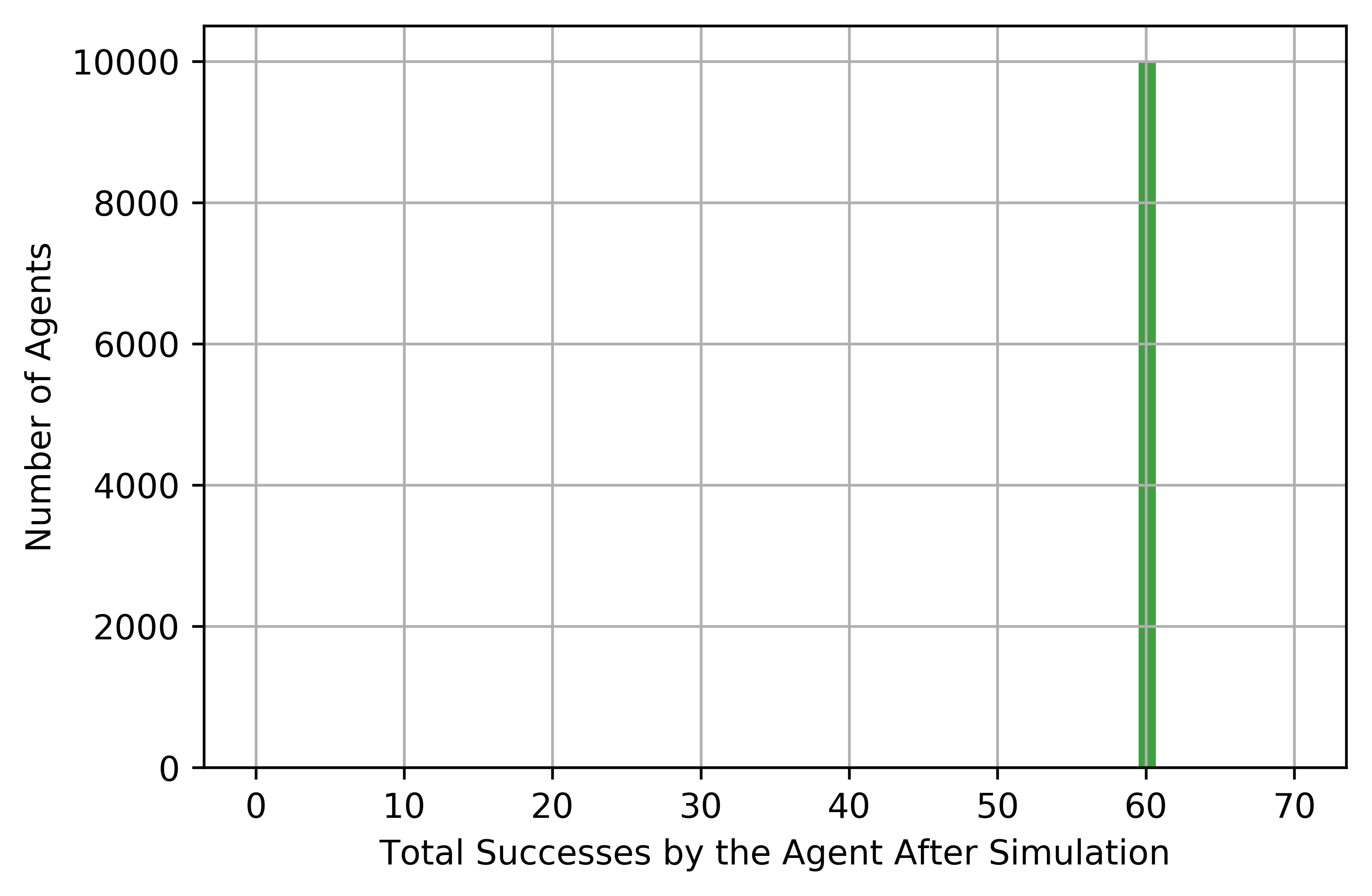 Pure-strategy Nash equilibrium attendance figures and agent success histogram over the 60 week simulation period, where everyone is supplied with the same random initial data for the first 20 weeks of traffic.
It is very important to note that most combinations of pure strategies among the agents do not produce a Nash equilibrium, and any uniform pure strategy applied by all the agents is bound to fail [1]. For example, if everyone’s strategy was to take the average of the previous week’s traffic then they would all predict the same attendance and act in the same way, which would inevitably lead to everyone being unhappy with their decision. For a more general problem involving mixed strategies it is also very unlikely that the total utility gets maximized, because it requires a level of coordination in the driver’s strategies that is infeasible without communication. However the Nash equilibria are still important as stable points of a dynamic adjustment process in which the drivers search for strategies that maximize their utility, even when the information available is minimal [6]. To reinforce this point we will now consider the situation where the drivers are maximally uncertain about the traffic numbers, so they resort to an entirely random guess about how many drivers will be on the road every week that ranges from $0$ to $N$.
Random Guesses About the Attendance
How many successful (i.e. utility-maximizing) choices do we expect each driver to make if they’re all guessing randomly? For the purposes of this blog we’ll use an intuitive but slightly hand-wavy approach which gives the right answer, but if you’re interested in a more rigorous analysis then I invite you to check out the attached Jupyter Notebook. Recalling that a driver decides to stay if they expect traffic to occur (i.e. their prediction is $\geq m$ total people on the road), there are $m$ predictions for which the driver decides to go $(0, \ldots, m-1 )$ and $N-m+1$ predictions for which they stay home $(m, \ldots, N)$. Thus the probability that an individual driver goes is $p = \frac{m}{N+1}$, and the probability that they stay is $1-p=\frac{N-m+1}{N+1}$. One shouldn’t be too concerned with the $+1$ in any of these formulas because it goes away as $N$ gets large. The expected number of people who go is then $p$ times the number of people who are considering going ($N$), so expected attendance is \begin{aligned} N\times\frac{m}{N+1} \to m \text{ as $N$ gets large}. \end{aligned} So for large $N$ the attendance based on random guesses fluctuates around the pure strategy Nash equilibrium attendance of $m$, with approximately equal probability of there being an attendance of $m+x$ as $m-x$, where $x$ is a small positive number. Mathematicians in the readership look away now, here’s where the real hand-waving occurs. When attendance is $> m$, then the fraction of people who maximize their utility is the fraction which stayed home, which has a typical value of $\frac{N-m}{N}=1-\frac{m}{N}$. When attendance is $< m$, the people who chose to go maximized their utility, making up $\frac{m}{N}$ of the people on average. Since the attendance is equally likely to be $> m$ or $< m$ in the large $N$ limit, the expected fraction of agent successes is \begin{aligned} \frac{1}{2}\bigg( \frac{m}{N}\bigg) + \frac{1}{2}\bigg( 1-\frac{m}{N}\bigg) = \frac{1}{2}. \end{aligned} For the 60-week simulation period that we are considering, this corresponds to an expected 30 successes per driver. Taking a look at the simulation results for $N = 10000$ and $m = 0.6N$, we find that our expectations are corroborated.
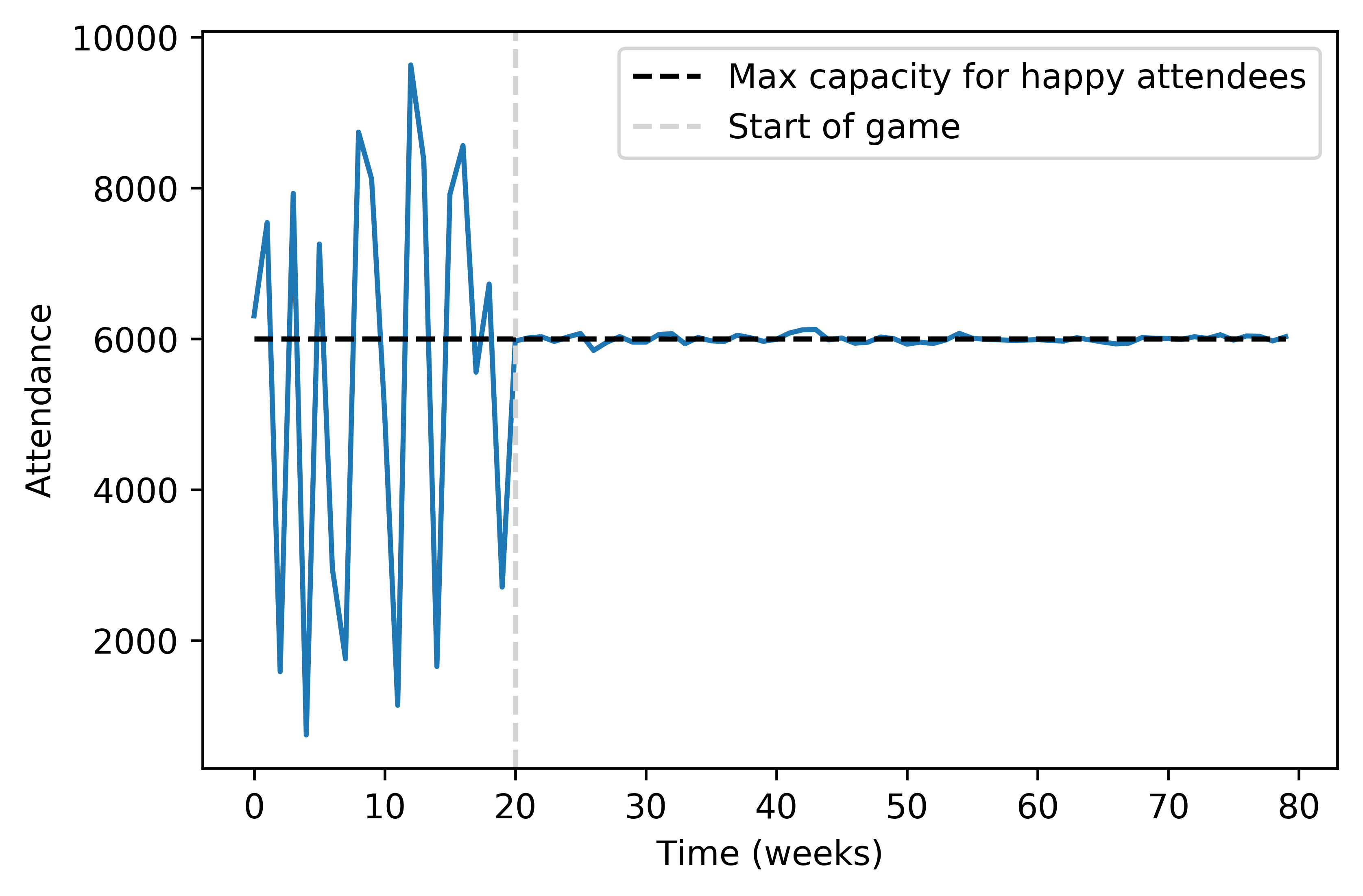
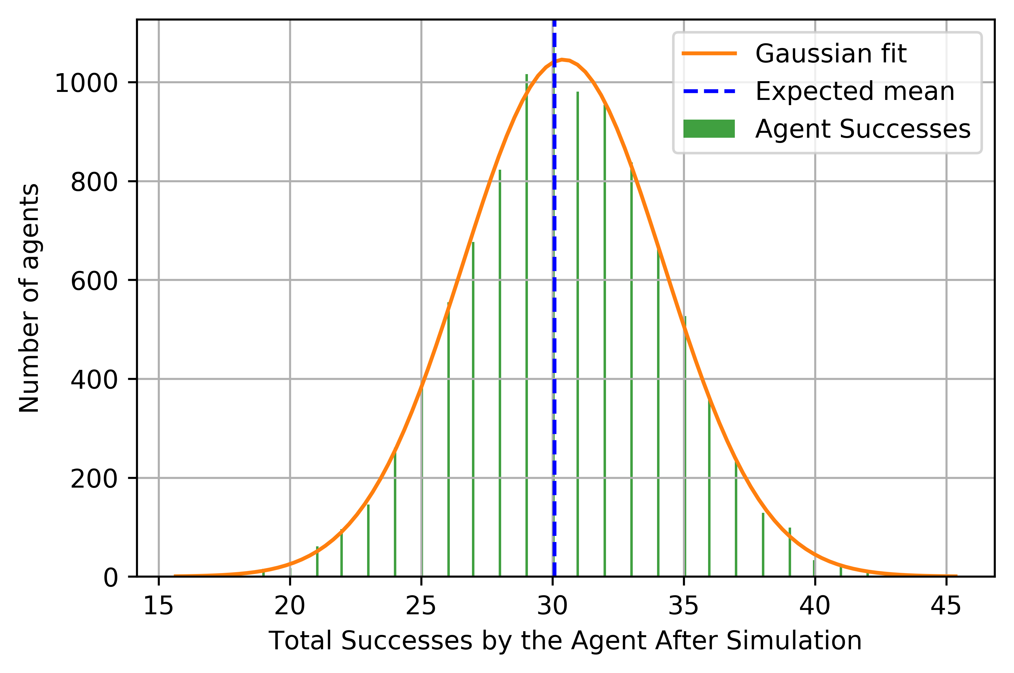 Attendance figures and agent success histogram over the 60 week simulation period, where each agent randomly guesses about the next week’s attendance and acts on those guesses. Note the blue line is an exact calculation of the expected number of successes for 10,000 agents (30.0651 to be specific), but for this particular simulation the mean successes were slightly higher than the expected value. Each agent is supplied with the same random initial data for the first 20 weeks of traffic.
There are two things I want to point out about the driver success histogram above. First, the number of successes per driver actually follows a binomial distribution, since each week the likelihood of success depends on the total number of drivers who show up independently on the day and each one drives with probability $p$. However, since $N$ is large the central limit theorem tells us that the Gaussian distribution is a good approximation for our distribution, which is why the data fits a Gaussian so well. Second, the random nature of the driver strategies means that the peak of the Gaussian fit fluctuates around the expected number of successes (blue line in the plot) for each simulation that you run, which is why the trial shown here has its peak at a slightly higher number of successes than the 30 we predicted. If you ran many trials and averaged the Gaussian peak locations, the answer would converge to the expected success number.
Full El Farol Bar Problem - Each Person Has $k$ Strategies to Pick From
This is all well and good, but what drivers do you know make a totally random guess about the traffic before they decide to go driving? Also if their guesses are completely wrong, you would expect them to change their strategy over time. Let’s let all hell break loose now and give each driver the full power of the original El Farol Bar Problem. We maintain $N = 10000$ and $m = 0.6N$ for this simulation, but at the beginning of the simulation each of the drivers are randomly assigned $k = 3$ of the $13$ possible pure or mixed strategies. Remember that a driver will switch their active strategy out for a different strategy available to them if they fail to maximize their utility with their current strategy for a given week. The results of the simulation are below.

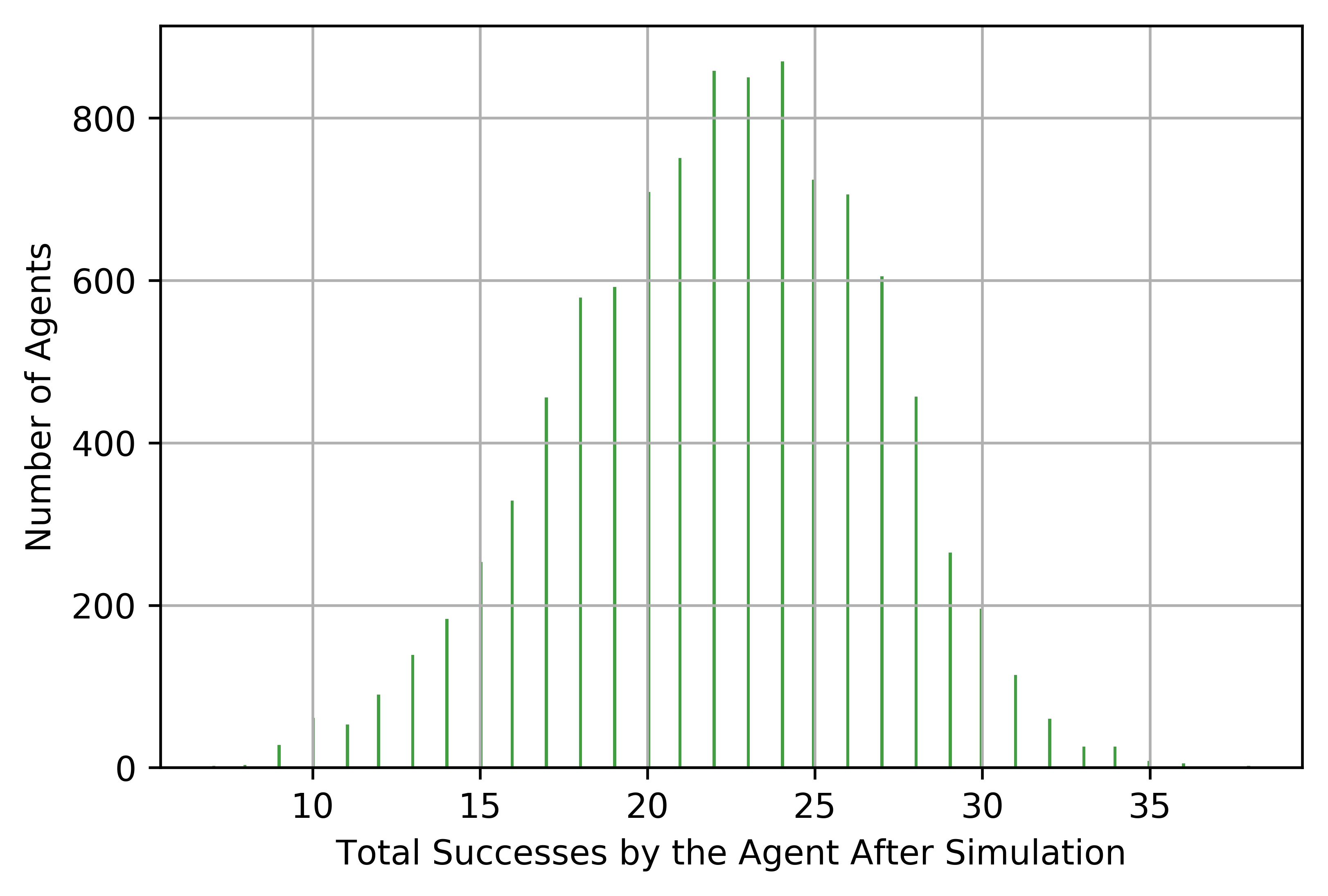 Attendance figures and agent success histogram over the 60 week simulation period for the full El Farol Bar Problem, where each agent aims to maximize their utility and has access to k possible strategies that they can switch between. Each agent is supplied with the same random initial data for the first 20 weeks of traffic. Notice that the success histogram now peaks below t/2=30 successes; compared to the situation with random guesses, the game is more competitive and there are fewer successes to be had on average.
Despite the fact that the agents apply very different strategies, the attendance still fluctuates around the pure strategy Nash equilibrium value like it did when everyone was making random guesses! Apparently giving agents the ability to change their strategy based on utility maximization does not prevent the system as a whole from self-organizing towards the stable point provided by the Nash equilibrium. Any patterns in attendance that some agents may pick up on and attempt to exploit are quickly stamped out by the rest of the field [1]. However, it should be noted that when compared with the random guesses simulation there is much higher variance in the El Farol simulated attendance figures. This goes hand in hand with the fact that the success histogram is now centered below $t/2=30$ successes: the game becomes significantly more competitive once the agents can change their strategy rather than being restricted to random guesses.
To reiterate a point made earlier, the general result of fluctuations around the pure strategy Nash equilibrium is not dependent on this particular instantiation of the El Farol Bar Problem with its specific list of strategies (and choices of $N$, $m$, $k$, etc.) - rather they hold for a large variety of game definitions (e.g. the minority game where $N$ players choose one of two sides and those on the minority side win) and payoff structures, including changing the learning models of the agents to something more realistic like stochastic adaptive learning [7].
Comparison to Real Traffic Data
All of these game theoretic simulations are certainly interesting, but do they really relate to traffic situations in the real world? As a point of comparison we can pull continuous data from CDOT (Colorado Department of Transportation) on an active road in Denver. Of course we can’t directly compare the results of our simulation with continuous data because there are daily periodic variations in the real traffic data, but if we pick a particular time to study then we can see what the day-to-day traffic fluctuations look like. Specifically I’ll use the 12 pm and 5 pm data from Interstate 70 East (Station 000511) over the months of January-March 2021, separating out the primary (P, east) and secondary (S, west) directions. The count data for a given time refers to the total number of cars that were counted over one hour starting at that time (e.g. starting at 12 pm and ending at 1 pm).
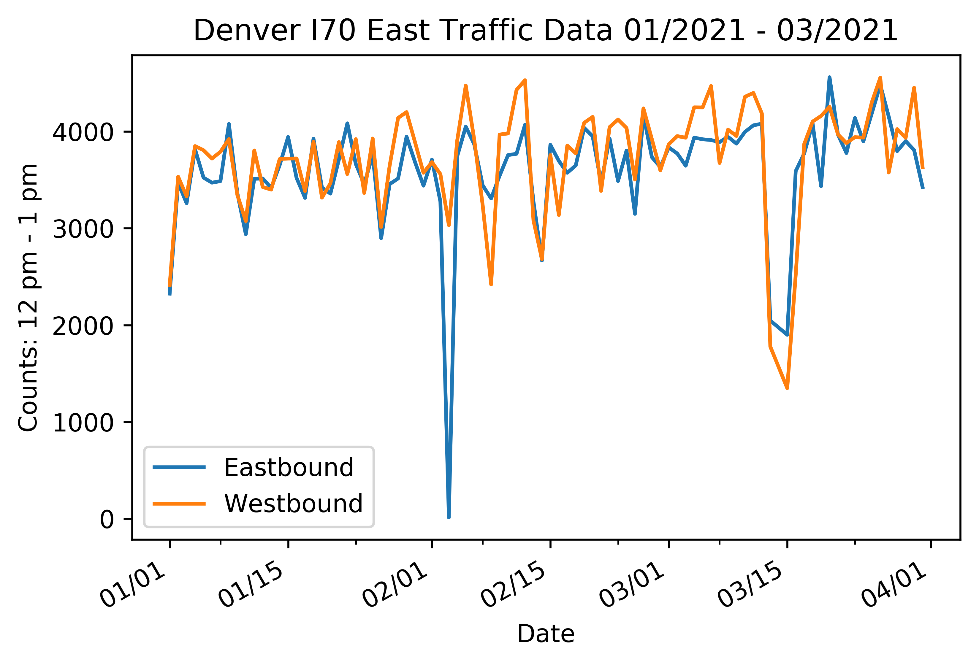
 Real traffic count data taken on I70 East in Denver. We choose here to look at the 12 pm - 1 pm (top) and 5 pm - 6 pm (bottom) data. All times are MST.
Remember that all of our simulations were initialized with 20 weeks of random data, so we should only compare the Denver traffic data above with the simulation results after the start of the game (weeks 20-80). Also recall that the only reason we represented the simulation duration in weeks was to match the framing of the original El Farol Bar Problem, but we could have easily called them day-to-day simulations simply by renaming the units on the horizontal axis. Thus we can compare the simulation results directly with the Denver day-to-day data. Qualitatively the real-life traffic numbers look quite similar to our El Farol simulation, with sizable fluctuations around an apparent equilibrium value, the “typical” occupation of Interstate 70 East at a given time of day. It is likely that this equilibrium value drifts seasonally, but it appears relatively fixed over this three-month period. One clear difference from our simulation is the major traffic dips recorded on February 3rd for the Eastbound 12 pm data and along both directions of traffic and during both times of day from March 13th through March 15th. The February 3rd dip was due to a large crash that occured before noon which shut down eastbound traffic on the interstate for several hours, which explains why the 5 pm eastbound data shows no dip on that day. The blanket drops in traffic from March 13th-March 15th were caused by a historic snowstorm that hit much of Colorado, but which was particularly centered around the Denver/Fort Collins region. Our El Farol simulation fails to account for such anomalous events when predicting traffic numbers.
To be more rigorous in our comparison we can look at the size of traffic fluctuations relative to the mean value for both the real data and our random guess and El Farol simulations. The standard deviation is a prima facie reasonable parameter to examine since it is a measure of a dataset’s dispersion, but it is not the best metric to use in this case because the real data and simulations have significantly different means. When you want to compare the dispersion of datasets with different units or substantially different means (and given that the mean is not close to zero and all data is positive, which is the case here), the coefficient of variation, or CV, is a better metric to use than the standard deviation [8]. The CV is a unitless quantity defined as the ratio of the standard deviation to the mean. Hence the smaller the CV, the closer the data lies to the mean.
Calculating the Denver traffic data’s CV for each direction and time, we get the following results:
| CV | |
|---|---|
| 12 pm Eastbound | 0.160 |
| 12 pm Westbound | 0.149 |
| 5 pm Eastbound | 0.173 |
| 5 pm Westbound | 0.182 |
Since attendance patterns vary for each simulation, I ran fifteen trials of the El Farol and random guess scenarios and calculated their CVs, and the average El Farol CV was 0.213 while the average random guess CV was 0.00812. The minimum and maximum CVs for the El Farol simulation were 0.189 and 0.243, and the min/max CVs for random guesses were 0.00649 and 0.00899. For how idealized and different the game theoretic El Farol model is from the complex world of real driving, it is impressive how similar the dispersion of the simulation’s attendance numbers is to that of real traffic (well within the same order of magnitude). By contrast the attendance based on random guess strategies is so much more tightly clustered than either the real data or the El Farol simulation, which is evident both from the attendance plots above and the random guess CV being approximately two orders of magnitude smaller than the others.
Conclusion
I want to end this blog post by pointing out multiple ways in which this toy model of traffic is wrong, and discuss model-building in general. As stated in the previous section, the El Farol model misses low-probability major events like crashes or inclement weather. One might attempt to realize such interruptions in the model by including a low probability for the bar capacity $m$ to drop to a small fraction of its typical capacity; the probability can be determined empirically for a given road with available traffic counter data from the observed interruption rate. Also, we assumed towards the beginning of the post that none of the drivers knew what the others were going to do, but nowadays with GPS-equipped cellphones everyone has access to information about the current state of traffic which can be used to inform your decision to drive. We also implicitly assumed that the drivers had the choice to stay home if they expected the traffic to be too bad, but someone in a rush is going to drive regardless of the traffic they expect. We could improve the model in a straightforward way by including some fraction of the population that does not adjust their strategy based on their predictions and let the remaining population act in the way we have simulated the agents here.
Although our model produced attendance numbers that were similar in their unpredictability to real traffic data at a fixed time of day, the model is not intended to describe the dynamics of traffic flow. One can divide traffic flow into two types [9, 10]:
- Free flow during light traffic, where cars drive at their maximum speed,
- Congested flow under heavy traffic conditions, where jam clusters or “stop-and-go waves” in which cars stop or move slowly propagate upstream (in the opposite direction as the motion of the cars).
Data from real expressways and indoor circuit experiments shows a dynamical jamming transition between these two types of flow at sufficiently high car density on the road, even in the absence of bottlenecks [9]. Several traffic models originating from a physics viewpoint produce the same vehicle flow rate/density relation observed in real traffic, including microscopic “follow-the-leader” models where each car is affected only by the vehicle ahead of it according to specific differential equations, kinetic models which idealize the cars as a gas of interacting particles, and macroscopic models where the cars are treated as a one-dimensional compressible fluid [10]. Interestingly, one can derive the macroscopic fluid model from the follow-the-leader model or kinetic gas model, and the phase transition and critical point predicted by these models correspond to those of a conventional gas-liquid phase transition [10].
Clearly our El Farol model can’t be used to predict what the actual traffic is going to look like day-to-day, and other models like the follow-the-leader or fluid models discussed above would be more appropriate for such predictions once paired with real measurements. The intention of this blog post was just to show how a simple model based on game theory can qualitatively reproduce the emergent traffic fluctuations that we actually see in everyday life. This is the aim of physics in a sense, the application of a highly simplistic model to better understand some behavior in the messy outside world by reducing that behavior to its essence. In this case the behavior of interest was the decision-making process that an individual applies when there is incomplete or unavailable information about how everyone else will act, such as when one decides whether or not to take a particular road on their morning commute or trip to the ski slopes. We learned that in such complicated scenarios humans will typically resort to inductive reasoning, where abstract mental models or strategies compete against one another based on a history of success or failure. And we saw how the El Farol Bar Problem posed by W. Brian Arthur in 1994 provides a solid framework for analyzing and simulating human inductive reasoning in situations like traffic, especially when converted into the language of game theory. So the next time that you find yourself stuck in traffic, don’t blame the other drivers. They’re all playing the same game as you, it just happens to be an easy game to lose.
References
[1] Arthur, W. Brian. “Inductive reasoning and bounded rationality.” The American economic review 84, no. 2 (1994): 406-411.
[2] Whitehead, Duncan. “The el farol bar problem revisited: Reinforcement learning in a potential game.” ESE discussion papers 186 (2008).
[3] Rumelhart, David E. Schemata: The building blocks of cognition. Routledge, 2017.
[4] Archibald, Erik, and Sue McNeil. “Learning from traffic data collected before, during and after a hurricane.” IATSS research 36, no. 1 (2012): 1-10.
[5] Chen, Shu-Heng, and Umberto Gostoli. “Coordination in the El Farol Bar problem: The role of social preferences and social networks.” Journal of Economic Interaction and Coordination 12, no. 1 (2017): 59-93.
[6] Holt, Charles A., and Alvin E. Roth. “The Nash equilibrium: A perspective.” Proceedings of the National Academy of Sciences 101, no. 12 (2004): 3999-4002.
[7] Papakonstantinou, Athanasios. “The El Farol Bar Problem for next generation Systems.” York: The University of York (2006).
[8] FAQ: What is the coefficient of variation? UCLA: Statistical Consulting Group. from https://stats.idre.ucla.edu/other/mult-pkg/faq/general/faq-what-is-the-coefficient-of-variation/ (accessed June 15, 2021).
[9] Tadaki, Shin-ichi, Macoto Kikuchi, Minoru Fukui, Akihiro Nakayama, Katsuhiro Nishinari, Akihiro Shibata, Yuki Sugiyama, Taturu Yosida, and Satoshi Yukawa. “Phase transition in traffic jam experiment on a circuit.” New Journal of Physics 15, no. 10 (2013): 103034.
[10] Nagatani, Takashi. “The physics of traffic jams.” Reports on progress in physics 65, no. 9 (2002): 1331.